Quantcast
Channel: C++博客-eryar
Viewing all 519 articles
Browse latest View live

OpenCASCADE点向圆柱面投影

$
0
0

OpenCASCADE点向圆柱面投影

eryar@163.com


OpenCASCADE的类Extrema_ExtPElS提供了点到基本曲面的投影计算功能,距离可能是最大值或是最小值。如下图所示的点到圆柱的投影会有两个投影点P1P2,则点到圆柱的距离的最小值是PP1的距离,最大值是PP2的距离。本文主要是对此类中点到圆柱的投影算法进行分析。


Extrema_ExtPElS类中计算点到圆柱的投影源码列出如下:


结合源码的注释可以看出点P到圆柱S的投影主要按有如下步骤:

l 计算点P到以圆柱S轴线为法线的平面的投影点Pp

l 若点P在轴线上,则计算失败返回;

l 计算点Pp在圆柱U方向的参数U1(角度);

l 将参数U1(角度)加180度得到参数U2

l 计算参数(U1V),(U2V)对应在圆柱面上的点;

上述实现主要也是使用向量的运算,所以程序简单且性能高。其中保存的距离是距离的平方值,这种方式主要考虑的是自带的开方函数性能,除非后面要用到距离才会自己去开方,这样也是提供性能的一种处理方式。

OpenCASCADE的向量类gp_Vec提供了一个函数AngleWithRef(),查看源码可知这个函数主要是计算两个向量之间的夹角,其中参数向量Ref是用来处理角度的正负。当两个向量叉乘的向量与参考向量Ref反向时,也会将得到的角度值取负。

下面通过一个简单的小程序来将计算结果在Draw Test Harness中可视化,这样可以直观地验证一下:


将生成的脚本文件加载到DRAW中得到如下图所示的结果:


从上图可以看出,投影得到的两个点P1P2的高度值与点P是相同的。


为了方便大家在移动端也能看到我的博文和讨论交流,现已注册微信公众号,欢迎大家扫描下方二维码关注。
Shing Liu(eryar@163.com)


eryar 2019-09-22 22:39 发表评论

OpenCASCADE 7.4.0测试版本发布

OpenCASCADE 平面求交

$
0
0

OpenCASCADE 平面求交

eryar@163.com


OpenCASCADE提供了类IntAna_QuadQuadGeo用来计算两个二次曲面quadric(球面、圆柱面、圆锥面及平面,平面是二次曲面的特例)之间的交线。他们之间可能的结果有:

l 一个点

l 一条或两条直线

l 一个点和一条直线

l 圆

l 椭圆

l 抛物线

l 双曲线


将源码结合《高等数学》、《解析几何》等书,可以来学习如何将理论付诸实践。本文主要介绍这个类中两个平面求交的源码实现。从源码中也可以看出OpenCASCADE官方开发人员的编码习惯。


将源码列出如下:

void IntAna_QuadQuadGeo::Perform (const gp_Pln& P1, 
                                  const gp_Pln& P2,
                                  const Standard_Real TolAng,
                                  const Standard_Real Tol)
{
  Standard_Real A1, B1, C1, D1, A2, B2, C2, D2, dist1, dist2, aMVD;
  //
  done=Standard_False;
  param2bis=0.;
  //
  P1.Coefficients(A1,B1,C1,D1);
  P2.Coefficients(A2,B2,C2,D2);
  //
  gp_Vec aVN1(A1,B1,C1);
  gp_Vec aVN2(A2,B2,C2);
  gp_Vec vd(aVN1.Crossed(aVN2));
  //
  const gp_Pnt& aLocP1=P1.Location();
  const gp_Pnt& aLocP2=P2.Location();
  //
  dist1=A2*aLocP1.X() + B2*aLocP1.Y() + C2*aLocP1.Z() + D2;
  dist2=A1*aLocP2.X() + B1*aLocP2.Y() + C1*aLocP2.Z() + D1;
  //
  aMVD=vd.Magnitude();
  if(aMVD <=TolAng) {
    // normalles are collinear - planes are same or parallel
    typeres = (Abs(dist1) <= Tol && Abs(dist2) <= Tol) ? IntAna_Same 
      : IntAna_Empty;
  }
  else {
    Standard_Real denom, denom2, ddenom, par1, par2;
    Standard_Real X1, Y1, Z1, X2, Y2, Z2, aEps;
    //
    aEps=1.e-16;
    denom=A1*A2 + B1*B2 + C1*C2;
    denom2 = denom*denom;
    ddenom = 1. - denom2;
    denom = ( Abs(ddenom) <= aEps ) ? aEps : ddenom;
    par1 = dist1/denom;
    par2 = -dist2/denom;
    gp_Vec inter1(aVN1.Crossed(vd));
    gp_Vec inter2(aVN2.Crossed(vd));
    X1=aLocP1.X() + par1*inter1.X();
    Y1=aLocP1.Y() + par1*inter1.Y();
    Z1=aLocP1.Z() + par1*inter1.Z();
    X2=aLocP2.X() + par2*inter2.X();
    Y2=aLocP2.Y() + par2*inter2.Y();
    Z2=aLocP2.Z() + par2*inter2.Z();
    pt1=gp_Pnt((X1+X2)*0.5, (Y1+Y2)*0.5, (Z1+Z2)*0.5);
    dir1 = gp_Dir(vd);
    typeres = IntAna_Line;
    nbint = 1;
    //
    //-------------------------------------------------------
    // When the value of the angle between the planes is small
    // the origin of intersection line is computed with error
    // [ ~0.0001 ] that can not br considered as small one
    // e.g.
    // for {A~=2.e-6, dist1=4.2e-5, dist2==1.e-4} =>
    // {denom=3.4e-12, par1=12550297.6, par2=32605552.9, etc}
    // So, 
    // the origin should be refined if it is possible
    //
    Standard_Real aTreshAng, aTreshDist;
    //
    aTreshAng=2.e-6; // 1.e-4 deg
    aTreshDist=1.e-12;
    //
    if (aMVD < aTreshAng) {
      Standard_Real aDist1, aDist2;
      //
      aDist1=A1*pt1.X() + B1*pt1.Y() + C1*pt1.Z() + D1;
      aDist2=A2*pt1.X() + B2*pt1.Y() + C2*pt1.Z() + D2;
      //
      if (fabs(aDist1)>aTreshDist || fabs(aDist2)>aTreshDist) {
        Standard_Boolean bIsDone, bIsParallel;
        IntAna_IntConicQuad aICQ;
        //
        // 1.
        gp_Dir aDN1(aVN1);
        gp_Lin aL1(pt1, aDN1);
        //
        aICQ.Perform(aL1, P1, TolAng, Tol);
        bIsDone=aICQ.IsDone();
        if (!bIsDone) {
          return;
        }
        //
        const gp_Pnt& aPnt1=aICQ.Point(1);
        //----------------------------------
        // 2.
        gp_Dir aDL2(dir1.Crossed(aDN1));
        gp_Lin aL2(aPnt1, aDL2);
        //
        aICQ.Perform(aL2, P2, TolAng, Tol);
        bIsDone=aICQ.IsDone();
        if (!bIsDone) {
          return;
        }
        //
        bIsParallel=aICQ.IsParallel();
        if (bIsParallel) {
          return;
        }
        //
        const gp_Pnt& aPnt2=aICQ.Point(1);
        //
        pt1=aPnt2;
      }
    }
  }
  done=Standard_True;
}

要理解这个源码,需要知道平面的一般方程:Ax+By+Cz+D=0,两个平面之间的夹角等概念。通过源码,可以看出计算两个平面之间的交线的步骤如下:

l 获取两个平面的一般方程的系数:ABCD,其中平面的法向量(A,B,C)为单位向量;

l 将两个平面的法向量叉乘得到的向量vd为平面交线的方向;

l 分别计算一个平面上的点到另外一个平面的距离:dist1dist2

l 如果向量vd的大小小于指定的精度TolAng,则认为两个平面平行没有交线;如果两个距离dist1dist2小于指定的精度Tol,则认为两个平面是相同的(重合);

l 计算两个平面的夹角denom

l 根据两个平面的夹角计算交线上的点;

l 后面是处理两个平面夹角很小的情况;

l 最后得到交线上的点pt1和方向dir1


其实上面求交线上点的代码不好理解,可以换成三个平面求交点的处理更好理解,如将交线的方向作为法向得到的一个平面与那两个平面一起计算交点,这个交点就一定在交线上,相关代码如下:

gp_Pln P3(vd.X(), vd.Y(), vd.Z(), 0.0);
IntAna_Int3Pln aTool(P1, P2, P3);
if (aTool.IsDone())
{
    pt1 = aTool.Value();
}

因为三个平面求交点是用高斯消元法解三元一次方程组,性能没有上面的代码好。生活中到处都是选择题,如何抉择是个问题啊。


为了方便大家在移动端也能看到我的博文和讨论交流,现已注册微信公众号,欢迎大家扫描下方二维码关注。
Shing Liu(eryar@163.com)


eryar 2019-10-07 19:38 发表评论

OpenCASCADE 平面与球面求交

最小二乘法拟合三维直线

$
0
0

最小二乘法拟合三维直线

eryar@163.com


在《高等数学》的书中给出了最小二乘法拟合直线的具体实例,但是那个例子是拟合二维直线的f(t)=at+b,那么三维直线怎么使用最小二乘法来拟合呢?我们先来看看《高等数学》书中的例子,由于任何实数的平方都是正数或零,因此我们可以考虑选取常数a, b,使


M最小来保证每个偏差的绝对值都很小,这种根据偏差的平方和为最小的条件来选择常数a, b的方法叫做最小二乘法(Least Square)。因为M是平方和,所以M的最小值在导数等于零的时候取得,即:


根据这个条件计算得到的最小值就是最小二乘解。因为拟合函数是二维直线方程f(t)=at+b是线性的,所以二维直线的拟合是线性最小二乘问题。对于三维直线,如果选择其代数方程,是两个平面的交线来表达的:


可以看出待确定的参数有8个,不是一个好办法。可以采用直线的参数表达,根据直线的对称式方程导出直线的参数方程:


我们要做的是根据N个采样点Pi确定参数方程的PD,使所有采样点到直线的距离的平方和最小。对于三维点到三维直线的距离我们可以使用矢量方法来计算,可以参考《点向直线投影》,


向量VP到采样点Pi的向量,向量D为直线的方向向量,是单位向量。VD点乘得到VD的投影长度,即图中红色标示部分的长度l。则采样点到直线的距离的平方是向量V的模的平方减去投影长度l的平方。从而得到采样点到直线的距离平方和方程:


参考“最小二乘法三维(k)直线拟合http://www.whudj.cn/?p=72”可知,最小二乘法拟合的直线通过所有采样点的中心点。即可以确定直线参数方程中的P。这样最小二乘方程就是只有方向矢量的一个多元函数。使用类math_MultipleVarFunctionWithGradient来建立上述最小二乘方程:


其中成员变量myPoint是直线的中心点,myPoints是所有的采样点。最小二乘方程为确定直线参数方程中的方向矢量(dx, dy, dz)的三个变量方程。使用math_BFGS之类的非线性极值计算类来对这个最小二乘方程进行求解。下面给出几个测试用例:


综上所述,拟合三维直线的最小二乘方程中点到直线的距离为点到直线的垂直距离,而书中二维直线拟合只是两个y值之间的差值:


图 点到直线的距离 (来自:https://zhuanlan.zhihu.com/p/36429715


上述拟合过程也可看出三维直线的拟合是一个非线性的优化问题,处理这类问题的一般步骤就是先建立目标方程,再使用相关优化求解类来对方程进行求解。


为了方便大家在移动端也能看到我的博文和讨论交流,现已注册微信公众号,欢迎大家扫描下方二维码关注。
Shing Liu(eryar@163.com)


eryar 2019-11-21 13:17 发表评论

RvmTranslator7.2

OpenCASCADE动画功能2

$
0
0

OpenCASCADE动画功能2

eryar@163.com


OpenCASCADE是一个开发平台,主要提供三维曲面和实体建模、CAD数据交换及可视化等功能。OCCT最适用于开发三维建模CAD软件、加工制造或测量(CAM)软件及数值仿真软件。对于一些加工制造软件,需要简单的动画仿真功能。本文主要就来说说OCCT的动画功能。

OCCT7.1.0版本引入了类AIS_Animation等用于实现动画功能的类。

https://www.opencascade.com/sites/default/files/documents/release_notes_7.1.0.pdf


并在Draw Test Harness中增加命令vanimation来测试动画功能。其类图如下所示:


根据类图可知,OCCT中的动画分两种形式:模型动画和视图动画。本文主要关注的是Draw Test Harness中的命令vanimation的一些参数设置对动画功能的影响。下图为Draw Test Harness中命令vanimation的帮助信息:


在命令的帮助信息中给了动画功能命令的详细说明。如动画的定义、视图(相机)动画、模型动画、增加回调函数及视频录制功能等。其中有两个参数会影响动画过程中视图的交互。这两个参数是:

l -freeLook:跳过视图动画,字面意思是动画的时候还可以对视图进行缩放、旋转等操作;

l -lockLoop:禁用交互,字面意思是锁定动画循环,动画过程中不能有交互,需要等待动画循环结束。

这两个参数的设置可以实现类似于OpenSceneGraph中的动画仿真功能,感觉像是多线程的动画。即模型动画过程中还可以对视图进行交互操作。


从上面的动画可以看出,当模型动画的过程中,还可以对视图进行交互操作,如缩放和旋转等。对于有这种功能需求的,可以参考Draw Test Harness中命令vanimation的具体代码实现。


为了方便大家在移动端也能看到我的博文和讨论交流,现已注册微信公众号,欢迎大家扫描下方二维码关注。
Shing Liu(eryar@163.com)


eryar 2019-12-05 17:37 发表评论

编译PySide

$
0
0

编译PySide

PySide是跨平台应用程序框架QtPython绑定版本。在20098月,PySide首次发布。提供和PyQt类似的功能,并相容 API。但与 PyQt 不同处为使用LGPL授权。

PySide的推出比pyQt晚很多,但也有些年头了。由于先前PySide项目不是很完善,又缺乏文档,所以其存在感不高。Pyside的诞生主要是Nokia(收购了TrolltechNokia当时是Qt的爸爸)与Riverbank Computing谈崩了的结果。Riverbank ComputingpyQt的开发商,对pyQt采用GPLv3协议。Nokia主动与Riverbank Computing展开了多轮协商,表示希望pyQt能添加对LGPL协议的支持,这样对于很多商业用户会更友好,何况你在pyQt里使用的也是我们LGPL协议版本的Qt,这个要求不过分吧。Riverbank Computing说我觉得不行。大概是觉得Riverbank Computing吃相难看,Nokia一气之下决定单干,于20098月发布了支持了LGPL协议的PySidepyQt的对标产品。然鹅,就算你是亲生的,刚生下来也打不过一个壮小伙子,何况你马上就要被过继出去了。。(滑稽2011年,NokiaQt的商业许可卖给Digia2012年,NokiaQt完全卖给Digia,后者在2012年年底推出了Qt5。遭遇人生的重大变故,PySide项目未来如何发展还是个未知数,更不要说支持Qt5了。反观pyQt,在Qt5推出的半年内(20136月)就发布了支持Qt5pyQt5。一边是生死未卜的只支持Qt4还不完善的主要依靠社区维护的PySide,一边是全面支持Qt4/Qt5的文档健全的pyQt,强弱悬殊,高下立判。好在Digia收购了Qt后,决定大力度支持Qt全方位发展,并于20149月将Qt分拆成一家独立全资子公司The Qt Company,后者于2016年在纳兹达克赫尔辛基上市。PySideQt5提供支持的计划也从2014年开始筹备,也就是2015年上马的Qt for Python项目,该项目开发的模块命名为PySide2,以表示与老一代PySide的不同。虽说加大了投入,该补的课也绕不开,PySide2Qt公司和Qt社区开发者的共同努力下,也只在20186月才正式发布了第一个版本,稳定性还是个问题。不过从01是最难的,后面就容易了,尤其最近发布的Qt 5.12 LTS释放了非常积极的信号,PySide2已经日趋完善,又是亲生的,还有LGPL开源协议的加持,今后PySide2有足够的理由成为Python开发者使用Qt的第一选择。(来自:https://www.zhihu.com/question/306793447

有了编译开源库OpenCASCADE等的经验,这些开源库的编译都可以自己动手解决。首先下载源码,由于国外网站现在访问速度很慢,可以找国内的镜像,像清华大学的开源软件镜像站就很好,内容很多,下载速度非常快。

https://mirrors.tuna.tsinghua.edu.cn/


 在如下地址下载PySide的最新版本源码:

https://mirrors.tuna.tsinghua.edu.cn/qt/official_releases/QtForPython/pyside2/


当然,如果不想自己编译,可以直接下载Qt官方编译好的程序先体验。根据官方文档,编译PySide主要是配置用到的第三方库,如libclangPython, CMake等,这些都可以从Qt的开发工具中下载到:

https://mirrors.tuna.tsinghua.edu.cn/qt/development_releases/prebuilt


下载好后,我喜欢将配置写在一个批处理文件中,如下所示:

@echo off
set path=%path%;D:\Qt\perl-5.20.3.3\perl\bin;D:\Python\Python37;D:\Python\Python37\Scripts;D:\Qt\Qt5.14.0\bin;
set LLVM_INSTALL_DIR=D:\Qt\libclang
python setup.py install --qmake=D:\Qt\Qt5.14.0\bin\qmake.exe --cmake=D:\Qt\cmake-3.8.0-win32-x86\bin\cmake.exe

启动Visual Studio的命令行工具,切换到pyside-setup文件夹中,运行批处理就可以了。当然编译要花点时间。编译好后,会自动安装到Pythonsite-packages里面。切换到例子文件夹,运行例子代码,出来下面的窗口说明编译成功了。


选择Python的原因是可以对应用程序提供二次开发功能,而且支持GUI的定制开发。原来也考虑过Tcl/Tk,即OpenCASCADEDraw Test Harness使用的脚本语言,自定义扩展简单。但是支持的功能也相对简单,且原生的Tcl不支持面向对象的开发。Python支持面向对象的概念,同是也是跨平台的。自己编译QtPySide可以根据需要,不编译Qt的一些模块,使程序尽量精简。


为了方便大家在移动端也能看到我的博文和讨论交流,现已注册微信公众号,欢迎大家扫描下方二维码关注。
Shing Liu(eryar@163.com)


eryar 2020-01-14 20:48 发表评论

Qt Python Scriptable Application

$
0
0
     摘要: Abstract. Python and C++ are in many ways as different as two languages could be: while C++ is usually compiled to machine-code, Python is interpreted. Python's dynamic type system is often cited as the foundation of its flexibility, while in C++ static typing is the cornerstone of its efficiency. C++ has an intricate and difficult compile-time meta-language, while in Python, practically everything happens at runtime.

Key Words. Qt, Python, Shiboken2, PySide2  阅读全文

eryar 2020-02-24 14:56 发表评论

OpenCASCADE Customize Highlighting

RvmTranslator7.3

PipeCAD之管道标准库PipeStd(4)

BRep Builder

$
0
0

BRep Builder

eryar@163.com


1 Introduction

BRep_Builder提供了创建、修改BRep模型的方法。使用这个类,你可以从底层自己构建BRep体,前提条件是你要对BRep模型的数据结构有一定理解。边界表示法BRep的重点在边界的定义,打开BRep_Builder的类图:


可以看到其中重载了很多UpdateEdge函数,每个UpdateEdge函数都修改了Edge中的几何数据,包括边界的定义数据。若能理解每个UpdateEdge函数,则对OpenCASCADEBREP数据结构就能理解了。本文主要介绍其中两个函数的用法:AddRemove

 2 Add Shape

BRep_BuilderAdd函数的字面意思是将一个Shape添加到另外一个Shape中。因这个函数的实现比较简单,把源码列出如下:


void TopoDS_Builder::Add (TopoDS_Shape& aShape, 
                          const TopoDS_Shape& aComponent) const
{
  // From now the Component cannot be edited
  aComponent.TShape()->Free(Standard_False);
  // Note that freezing aComponent before testing if aShape is free
  // prevents from self-insertion
  // but aShape will be frozen when the Exception is raised
  if (aShape.Free())
  {
    static const unsigned int aTb[9]=
    {
      //COMPOUND to:
      (1<<((unsigned int)TopAbs_COMPOUND)),
      //COMPSOLID to:
      (1<<((unsigned int)TopAbs_COMPOUND)),
      //SOLID to:
      (1<<((unsigned int)TopAbs_COMPOUND)) |
      (1<<((unsigned int)TopAbs_COMPSOLID)),
      //SHELL to:
      (1<<((unsigned int)TopAbs_COMPOUND)) |
      (1<<((unsigned int)TopAbs_SOLID)),
      //FACE to:
      (1<<((unsigned int)TopAbs_COMPOUND)) |
      (1<<((unsigned int)TopAbs_SHELL)),
      //WIRE to:
      (1<<((unsigned int)TopAbs_COMPOUND)) |
      (1<<((unsigned int)TopAbs_FACE)),
      //EDGE to:
      (1<<((unsigned int)TopAbs_COMPOUND)) |
      (1<<((unsigned int)TopAbs_SOLID)) |
      (1<<((unsigned int)TopAbs_WIRE)),
      //VERTEX to:
      (1<<((unsigned int)TopAbs_COMPOUND)) |
      (1<<((unsigned int)TopAbs_SOLID)) |
      (1<<((unsigned int)TopAbs_FACE)) |
      (1<<((unsigned int)TopAbs_EDGE)),
      //SHAPE to:
      0
    };
    //
    const unsigned int iC=(unsigned int)aComponent.ShapeType();
    const unsigned int iS=(unsigned int)aShape.ShapeType();
    //
    if ((aTb[iC] & (1<<iS)) != 0) {
      TopoDS_ListOfShape& L = aShape.TShape()->myShapes;
      L.Append(aComponent);
      TopoDS_Shape& S = L.Last();
      //
      // compute the relative Orientation
      if (aShape.Orientation() == TopAbs_REVERSED)
        S.Reverse();
      //
      // and the Relative Location
      const TopLoc_Location& aLoc=aShape.Location();
      if (!aLoc.IsIdentity())
        S.Move(aLoc.Inverted());
      //
      // Set the TShape as modified.
      aShape.TShape()->Modified(Standard_True);
    }
    else {
      throw TopoDS_UnCompatibleShapes("TopoDS_Builder::Add");
    }
  }
  else {
    throw TopoDS_FrozenShape("TopoDS_Buider::Add");
  }
}


Add函数通过一个静态的检查列表,来检查添加的Shape是不是合法的,即FACE只能添加到SHELLCOMPOUND中,EDGE只能添加到WIRESOLIDCOMPOUND中等。添加之后还检查了ShapeORIENTATION及位置信息并作相应调整。不满足条件的情况都会抛出异常,所以对于Add函数需要增加异常处理逻辑。

使用这个函数需要注意的是这个Add只是简单的将Shape添加到TShapeShape表中,并没有维护BREP的边界信息。

3 Remove Shape

Add对应的有Remove函数,可以从一个Shape中删除一个子Shape。还是打开源码,有源码有真相:

//=======================================================================
//function : Remove
//purpose  : Remove a Shape from an other one
//=======================================================================
void TopoDS_Builder::Remove (TopoDS_Shape& aShape, 
                             const TopoDS_Shape& aComponent) const
{
  // check  if aShape  is  not Frozen
  TopoDS_FrozenShape_Raise_if (!aShape.Free(),"TopoDS_Builder::Remove");
  // compute the relative Orientation and Location of aComponent
  TopoDS_Shape S = aComponent;
  if (aShape.Orientation() == TopAbs_REVERSED)
    S.Reverse();
  S.Location(S.Location().Predivided(aShape.Location()));
  TopoDS_ListOfShape& L = aShape.TShape()->myShapes;
  TopoDS_ListIteratorOfListOfShape It(L);
  while (It.More()) {
    if (It.Value() == S) {
      L.Remove(It);
      aShape.TShape()->Modified(Standard_True);
      break;
    }
    It.Next();
  }
}


从源码中可知,Remove实现的逻辑也是很简单的:

检查Shape是不是Free的,若不是则抛出异常;

计算要删除ComponentORIENTATIONLOCATION

Shape列中查找Component,若找到将其从列表中删除;


删除操作比添加操作要简单,一个是把已有的数据删除,一个是从无到有的构建数据。从函数实现代码来看,删除操作也是简单的从Shape列表中删除指定的Shape。删除之后多余的边界信息还会存在原来的Shape中,要确保删除的Shape之后没有多余信息,还需要删除没有使用的PCurves


上图所示为删除一个底面的圆柱体。

 4 Conclusion

BRep_Builder的操作需要以充分理解OpenCASCADEBREP数据结构为前提,因为其AddRemove函数并没有提供维护边界的功能,只是将指定的Shape添加到列表中或从列表中删除。


为了方便大家在移动端也能看到我的博文和讨论交流,现已注册微信公众号,欢迎大家扫描下方二维码关注。
Shing Liu(eryar@163.com)


eryar 2020-06-16 11:04 发表评论

PBR in OCCT 3D Viewer

$
0
0

Forthcoming OCCT 7.5.0 release extends its real-time rendering engine with a PBR (physically-based rendering) mode. OCCT implements PBR metal-roughness material workflow described by core glTF 2.0 specifications and also includes glTF data exchange components. New functionality opens a door to a new level of realism and visual quality of displayed models, and improves interoperability across various 3D engines supporting the same material workflow.

Common material workflow

Before going forward to new PBR capabilities, let's take a look at a shading model available in previous versions of OCCT 3D Viewer.

The Phong/Gouraud reflection model has been widely used in real-time graphics for a long time. Thanks to its simplicity, convincing look and affordable performance, this model has been implemented by fixed-function Transformation & Lighting (T&L) hardware blocks on graphical cards of the past. Introduction of programmable pipeline with first GPUs has given more flexibility to application developers, providing nice improvements like switching from per-vertex (Gouraud) to per-fragment (Phong) shading.

Per-vertex (left) vs. per-fragment (right) shading.

Common (Phong) material model consists of the following components (see Graphic3d_MaterialAspect and XCAFDoc_VisMaterialCommon structures):

  • Ambient color (a constant multiplied by active light);
  • Diffuse color (main object color reflected);
  • Specular color (hotspot of the light on the object);
  • Emissive color (added regardless of active light);
  • Shininess factor (defines a size of light hotspot);
  • Transparency factor.

Components of Phong material model.

Phong shading is an empirical illumination model, which means that it does not try to comply with physical laws of light distribution. Even more, in pursuit of better visual appearance, material workflow implies the lighting environment to be partially baked into an object's material. Dynamic lighting remains computed in real-time, but the object’s material, being artistically prepared for a specific environment, looks natural only there and has to be adjusted for another environment.

PBR Metal-roughness material workflow

The limitations of conventional shading models and growing power of GPUs have pushed developers to look for better and more universal models.

Physically-Based Rendering (PBR) illumination models aim to fit surface shading formulas into constraints of physical laws of light propagation / absorption / reflection - hence called "physically-based". This comes to the concept of energy conservation, which states that an object can not reflect more light than it receives.

Various PBR engines define different material models, but metallic-roughness PBR material workflow became most commonly used thanks to several game engines implementing it and open glTF 2.0 3D asset exchange format specification relying on this model. A common material model is a good step forward to interoperability across engines, so that 3D artists now can be sure that their models look consistent and as designed. There is still some diversity across engines, like PBR specular glossiness material workflow, though.

Compared to Phong shading, PBR model relies on even smaller number of key material properties (see Graphic3d_PBRMaterial and XCAFDoc_VisMaterialPBR structures):

  • Base color (or albedo);
  • Emissive color (added regardless of light);
  • Metallic flag (switching between metal and dielectric properties);
  • Roughness factor (the level of material polishness);
  • Transparency factor.

Metal-roughness PBR material properties.

Emissive color has the same meaning as in case of a Phong shading, as it is applied regardless of lighting - its purpose is defining a cheap fake light source baked into an object.

Base color has a meaning very close to diffuse color in Phong shading. The latter one, however, may include baked properties like self-shadow, inappropriate to a clean albedo texture. Therefore, diffuse texture from Phong material can be passed directly to the PBR pipeline, but to eliminate visual artifacts an artist should manually preprocess texture and clean up from unexpected content.

Roughness factor defines microsurface material properties. Roughness can be considered as the opposite to polishness (or to glossiness, used by another PBR material model).

Metallic flag defines whether material should behave as metal or as dielectric while responding to the light. In real life, material should be either metal or non-metal, but PBR material workflow supports metallic factors in-between. Such values can be used for displaying a smooth material transition on boundaries - like from corrugated to non-corrugated metal. Usage of non-binary metallic values is discouraged in any other cases, as it may cause unexpected visual results.

With some practice, it soon becomes clear that defining an artistic PBR Metallic-Roughness material is much simpler than defining a similar material for Common material workflow. And unlike Phong shading, the material will behave reasonably in various environments within a proper PBR engine. This also allows the same model to be displayed correctly in different 3D engines.

Exact conversion between Common and PBR metal-roughness material models is impossible. But some material properties have close relations like diffuse color and albedo, shininess and roughness, so that a non-exact lossy conversion is provided by OCCT.

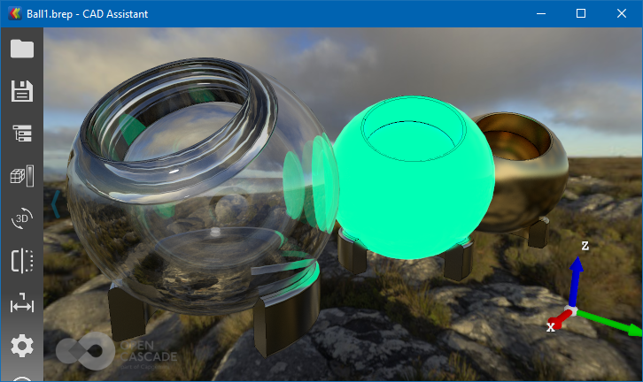
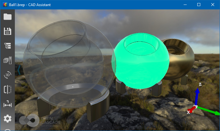
A special care must be taken while defining transparent materials in PBR. First of all, semi-transparent metal makes no sense from a physical point of view. For this reason, applying synthetic transparency might give unexpected results - it is desired resetting material metalness to zero for a natural look. One more material parameter affects transparency - Index of Refraction (IOR).

Additional texture maps

PBR models may be accompanied by base color (albedo) and metal-roughness texture maps, which meaning is clear. In addition, the following texture maps are supported by OCCT and defined by glTF 2.0 core specification:

  • Emissive map (adds color regardless of lighting);
  • Normal map (adds small surface details without extending geometry);
  • Occlusion map (defines a pre-baked global illumination).

As these extra maps have no direct relationship to PBR metal-roughness material workflow, OCCT 3D Viewer now supports these texture maps in both PBR and Phong shading models.

Normal texture may add extra details like scratches or imprints
without altering geometry.

Occlusion texture adds pre-baked global illumination
(smooth shadows at geometry corners).

PBR renderers in OCCT

OCCT provides two PBR renderers:

  • Cinematic non-real-time renderer (ray-tracing/path-tracing);
  • Real-time renderer (rasterization).

Cinematic renderer is designed for uncompromised quality, for which it relies on ray-tracing rendering pipeline (Graphic3d_RM_RAYTRACING). Performance of current graphics hardware does not make it possible using computationally-intensive path-tracing renderer in real-time graphics, but with some limitations it can be used in an interactive fashion. OCCT includes a Path-Tracing rendering engine since 7.0.0 release, and implemented using GLSL programs.


Photorealistic Path-Tracing (above) vs. real-time PBR (below)
rendering engines in OCCT.

The objective of real-time PBR renderer is to be fast enough even on low-end graphics hardware. For that, it heavily relies on traditional rasterization rendering pipeline (Graphic3d_RM_RASTERIZATION), various approximations and tricks making it applicable in real-time, while looking good enough and preserving most important physical properties.

OCCT 7.5.0 introduces a real-time PBR renderer supporting metal-roughness material workflow. The math behind OCCT renderer can be found directly in OCCT documentation. Current implementation handles transparent materials taking an Index of Refraction into account; more advanced transparent material properties might be considered in the future.

The math requires light computations to be done in linear color space, while computer displays use non-linear color space reflecting properties of the human eye. For this reason, OCCT renderer has been improved to handle properly sRGB/RGB color conversions. This has been done as a general improvement affecting not only new PBR renderer, but the Phong shading model, RGB color definition (Quantity_Color) and color import/export in Data Exchange components (STEP, IGES, glTF, OBJ, etc.).

The Path-Tracing engine relies on a more advanced BSDF (Bidirectional Scattering Distribution Function) material model (Graphic3d_BSDF), so that auxiliary conversion tools have been introduced. In particular, built-in OCCT materials have been updated to support PBR metal-roughness material by conversion from previously defined BSDF material properties.

New renderer extends the list of shading models (Graphic3d_TypeOfShadingModel enumeration) with Graphic3d_TOSM_PBR/Graphic3d_TOSM_PBR_FACET values. This makes it possible to mix objects with Phong, Unlit and PBR materials in a single scene, though results might be unexpected.

This is because apart from different material properties, PBR rendering has one more important difference compared to Phong shading - light source intensity. Within Phong shading, light sources have color values within normalized [0; 1] range - so that both a sun and a tiny lamp would have comparable color values in the scene. Obviously, this contradicts physical laws, and PBR introduces unnormalized light intensity property - which should be scaled according to an energy emitted by a light source in the real world.

Therefore, a proper light sources setup becomes more critical in PBR workflow and requires more attention. Exactly the same light source definition applied to PBR and Phong shading models produces different results due to unnormalized / normalized light intensity definition.

Image-based lighting

A good light sources’ setup is crucial for a nice-looking PBR rendering results, and it might become a problem. Directional light sources give only a small hotspot on metals, while uniform ambient light sources result in too whitish results, which is no good.

Much better results give an Image-Based Lighting (IBL) - an environment (ambient) lighting based on a predefined image. OCCT 7.4.0 introduced support of cubemaps for viewer background, and OCCT 7.5.0 PBR renderer uses this image background for a realistic environment lighting effect.

No ambient light (top-left), uniform white ambient (top-right),
white room environment (bottom-left) and lake environment (bottom-right).

So far, OCCT does not come with any environment maps, and application developers are responsible for providing them to OCCT 3D Viewer. Normally, an application should provide a list of such images in settings, as different models might look better / more natural in different environments.

Point light sources are handled physically by PBR renderer, so that their attenuation has a squared distance dependency and constant/linear attenuation factors (supported by Phong shading) are ignored. In addition, point light now provides an optional cut-off distance at which light source should be fully attenuated - this is not physically correct (realistic light has an infinite zero attenuation distance), but artistic/optimization feature allowing to manage numerous point sources in a scene.

Performance comparison

Real-time PBR renderer uses various approximations, a lookup table and special textures for Image-Based Lighting pre-baked from an environment image - the generation of these maps, and optimizations of generation of these maps can be considered as subject for a dedicated article. Even with all these tricks, PBR is considerably more computationally intensive than conventional Phong shading.

It is clear that switching from Phong to PBR will affect performance, but to which extent? Well, practically speaking, this is not that crucial on modern graphics hardware. First of all, it should be noted that the main computational complexity resides in a Fragment Shader, while a vertex processing part remains the same. This gives a nice quality to renderer - performance depends more on a frame buffer resolution rather than on a number of triangles.

Tests on modern desktop and mobile hardware show framerate drop from 0% to 15%, but older hardware and extra conditions might give more considerable slowdown.

Data Exchange

XCAF document structure has been extended with a new element - visualization material (XCAFDoc_VisMaterial). It should not be mistaken with previously defined material element (XCAFDoc_Material) defining physical properties (e.g. density).

Visualization material can define Common XCAFDoc_VisMaterialCommon (obsolete), PBR Metal-roughness XCAFDoc_VisMaterialPBR (new) properties, or both at the same time. This gives application flexibility to either rely on automatic conversion between material models or to define specific properties (as automatic conversion can give undesirable results).

The document defines a plain list of Visualization materials, which are assigned to specific parts or sub-shapes. Data Exchange components have been improved to use new elements:

  • XBF document stores any combination of material and color labels. It should be noted, however, that assigning both color and material to the same part gives not well defined result and should be avoided.
  • STEP, IGES and similar formats storing only color information keep using a color table in an XCAF document. Visualization materials in the document are exported as colors.
  • JT reader/writer now translates material properties into a Common material definition in an XCAF document.
  • glTF reader/writer now translates material properties into PBR material definition in an XCAF document.

XCAFPrs_Style now stores both color and visualization material properties, XCAFPrs::CollectStyleSettings() collects overwhelming information from the document and XCAFPrs_AISObject supports displaying visualization material.

Conclusion

PBR dramatically improves the visual quality of rendered models at minor performance costs (on modern hardware). It is not limited to use cases, where realistic look is crucial - PBR is universal and can be used in a wide range of scenarios, from CAD to cartoon animations.

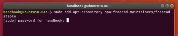
OCCT 3D Viewer supports a wide range of platforms and brings PBR renderer to desktop, mobile and web platforms. The minimal requirement is OpenGL 3.0+ or OpenGL ES 3.0+ capable hardware.
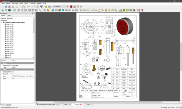
Metallic-roughness material workflow improves interoperability with other 3D engines supporting this workflow and ensuring consistent look of a model. Built-in glTF 2.0 data exchange component allows easily transmit models between OCCT and other systems like Blender.


A sample glTF model displayed in CAD Assistant, Blender and three.js
with close environment setup.

Materials in Draw Harness

The following tcl script defines a sample scene using Phong and PBR shading models.

pload OCAF XDE MODELING VISUALIZATION
vinit View1 -w 350 -h 400
# create an XCAF document from a sample model
restore [locate_data_file Ball.brep] ball
XNewDoc Doc
XAddShape Doc ball 0
# define a sample Common material
vrenderparams -shadingModel PHONG
XAddVisMaterial Doc matCommon -shininess 0.5 \
  -ambient DARKSLATEBLUE -diffuse CORNFLOWERBLUE \
  -specular WHITE
XSetVisMaterial Doc ball matCommon
XDisplay -dispMode 1 Doc
vfit
# define a sample PBR material
vrenderparams -shadingModel PBR
vlight -clear
vlight -add AMBIENT -intensity 1
vlight -add DIRECTIONAL -intensity 5 -headlight -direction 0 0 -1
XAddVisMaterial Doc matPbr -metallic 1 -roughness 0.5 \
  -albedo CORNFLOWERBLUE
XSetVisMaterial Doc ball matPbr
XDisplay -dispMode 1 Doc
vfit
# use cubemap for better ambient lighting
#vbackground -cubemap cubemap.png


eryar 2020-07-19 08:53 发表评论

IsoAlgo Symbols

$
0
0

IsoAlgo Symbols

eryar@163.com


Key Words. IsoAlgo, ISO, PCF, IDF, 管道轴测图


1. Introduction

管道轴测图(ISO图)是管道制作安装所需的重要图纸,其中管件符号是固定大小,管子长度可变的一种非比例投影的出图形式。目前国际出图标准程序是IntergraphISOGEN

鉴于ISOGEN是生成管道ISO的工业标准,其数据文件格式也基本上是工业软件生成的标准数据交换格式。主流工厂设计软件如Intergraph, AVEVA等都可以生成ISOGEN识别的管道数据文件PCFIDF

IsoAlgo是自主开发用于生成管道ISO图的程序,因为是做ISOGEN类似的功能,所以需要兼容ISOGEN的数据。对程序IsoAlgo进行代码重构,使其能支持ISOGEN的管道数据文件IDFPCF,并能支持符号模板文件,避免用户自定义符号,而且普通用户一般不需要自定义符号。通过支持ISOGEN的符号,使用户在默认状态下能生成与ISOGEN一致的管件符号。


2. Symobl Template

ISOGEN程序中管件的符号数据是一种模板形式的,且支持符号的自定义。符号数据文件的格式相对简单,主要数据为定义符号的形状。通过兼容ISOGEN的符号模板数据,避免用户自定义符号,且生成的ISO管件符号与ISOGEN一致。

3. Conclusion

集成IsoAlgoPipeCAD中方便测试,可实时查看生成结果。通过兼容ISOGEN的符号数据文件,可以生成与ISOGEN风格一致的ISO效果。因为ISOGEN的符号数据文件中包含了常用的符号模板,避免用户自定义符号。

通过兼容ISOGEN的数据,还可以尽量去猜测ISOGEN的出图算法,有一定的参考价值。下面几个ISO图为兼容ISOGEN符号数据生成的:


为了方便大家在移动端也能看到我的博文和讨论交流,现已注册微信公众号,欢迎大家扫描下方二维码关注。
Shing Liu(eryar@163.com)


eryar 2020-08-10 20:47 发表评论

[转]How to Install FreeCAD 0.18 in Ubuntu 18.04 / 16.04

$
0
0

FreeCAD, free and open-source 3D parametric modeler, released version 0.18 recently with Python 3 and Qt 5 support. Here’s how to install it in Ubuntu 16.04, Ubuntu 18.04, and Ubuntu 19.04.

FreeCAD 0.18 release highlights:

  • Extended TechDraw tools
  • New sketcher tools, more stable and robust PartDesign
  • Enhanced and extended Arch and BIM tools
  • Redesigned Start center
  • New Navigation Cube
  • Specify a custom background image for FreeCAD’s main window

Install or Upgrade FreeCAD in Ubuntu:

The official FreeCAD PPA has built the latest release packages for Ubuntu 16.04, Ubuntu 18.04, Ubuntu 19.04, and their derivatives.

1. Open terminal either via Ctrl+Alt+T keyboard shortcut, or by searching for ‘terminal’ from app menu. When it opens, run command to add the PPA:

sudo add-apt-repository ppa:freecad-maintainers/freecad-stable

Type user password (no asterisk feedback) when it prompts and hit Enter to continue.

2. If a previous release was installed on your system, upgrade it via Software Updater:

Or install the software via following commands:

sudo apt update

sudo apt install freecad

Uninstall:

To remove FreeCAD, simply run command in terminal:

sudo apt remove --auto-remove freecad

To remove the PPA, open Software & Updates -> Other Software.

转自:http://ubuntuhandbook.org/index.php/2019/04/install-freecad-0-18-ubuntu-18-04-16-04/


eryar 2020-09-09 10:58 发表评论

RvmTranslator 3D PDF in Ubuntu

$
0
0

eryar@163.com


RvmTranslator can translate the RVM file exported by AVEVA Plant(PDMS)/AVEVA Marine to STEP, IGES, STL, DXF, 3D PDF, OBJ, 3DXML, IFC,.etc. So it can be used for exchanging model data between other CAD software, such as Autodesk AutoCAD, Plant3d, 3ds Max, CATIA, Solidworks, Pro/E, Unity3d, .etc.

RvmTranslator可以将AVEVA PDMS/Plant/Marine中导出的RVM文件进行可视化,以及将RVM转换成常见的三维文件格式。如STEPIGESSTLDXF, OBJ, 3DPDF, 3DXML, IFC等,便于与其他CAD系统进行数据交换,如Autodesk AutoCAD, Plant3d, 3ds Max, CATIA, Solidworks, Pro/E, Unity3d, Bentley等。


由于使用的是跨平台的Qt等开源库,现在将RvmTranslator移植到Linux系统中,如下图所示为RvmTranslatorUbuntu系统中的界面:


RVMAVEVA的一个统一模型格式,包括其收购的船舶系统Tribon也可以导出RVM格式的文件。


上图为船舶管路,因为船体空间相对狭小,船舶管路布置的密集些。


Ubuntu中安装Adobe Reader才能显示3D PDF中的内容。Adobe Reader是免费软件,但是Ubuntu中没最新版本的,从这里下载最新版本9.5.5

ftp://ftp.adobe.com/pub/adobe/reader/unix/9.x/


在Ubuntu的Adobe Reader显示三维模型:


最后再来两个动图:


为了方便大家在移动端也能看到我的博文和讨论交流,现已注册微信公众号,欢迎大家扫描下方二维码关注。
Shing Liu(eryar@163.com)


eryar 2020-09-16 11:54 发表评论

OpenCASCADE STEP Color

$
0
0

OpenCASCADE STEP Color

eryar@163.com


Abstract. STEP AP214STEP中是带有颜色信息的,OCCT可以读取其中的颜色信息。本文介绍一种比官方XCAFDoc_ColorTool更方便的获取方法。

Key Words. OCCT, STEP, Color

1. Introduction

STEP是通用格式,常用的3D软件都可以打开,用于不同的软件之间相互交流之用。OCCTData Exchange模块支持STEP格式的读写功能,其中支持STEPAP203AP214版本,这两者有什么区别呢?下面从网上摘取如下解释:

应用协议(APs: Application Protocol)是用来交换数据。每种应用协议属于一个不同的应用领域。例如,AP227属于空间装置技术和包含几个实体属于这个区域,如管道Pipe或弯头Elbow。此外,这些APs使用某些公共实体称为通用资源,如几何和拓扑结构,定义实体模型。

AP203适用于机械零件和组件的表示。AP214适用于数据的表示有关汽车设计。今天AP203文件通常包含边界表示模型、装配数据和数量有限的其他产品信息。

AP214文件通常包含颜色,,和通用资源。边界表示法的模型是一个CAD模型代表它的边界。例如,一个表面模型由只有表面使用,使模型。固体模型包括几何信息,如表面,曲线,并指出,和拓扑信息,比如边缘,顶点,面临着。几何信息提供了数据模型的形式,和拓扑信息提供这些几何元素之间的连接性和几何元素的程度。

相同点:AP214 AP203均支持的实体、面的输入和输出。

区别是:STEP AP203 标准不具有任何颜色,AP214标准具有颜色的。

缩上所述,当以AP203应用协议保存STEP后,只保存了几何模型,没有颜色数据。当需要在STEP中体现颜色,就需要以AP214来保存。

为了更好的显示STEP模型或者需要将STEP中的模型及颜色转换到其他格式,需要获取STEP中的颜色信息。本文主要介绍如何在OCCT中读取AP214STEP中的颜色信息。

2. STEP in Draw

Draw Test Harnes中对应AP203AP214分别有两个命令来读取STEP文件:

l stepread:对应AP203协议,只读取STEP中的模型;

l ReadStep:对应AP214协议,能读取STEP中的模型、颜色、组装结构等;

通过命令ReadStep读取进来的模型,可以显示颜色:


ReadStep命令提示中可以看出,读取AP214的STEP需要用到OCCT的应用程序框架中的文档。即需要使用Extended Data Exchange(XDE)来读取。


3. Access STEP Color

XDE中可以读写模型的颜色信息,支持的三种颜色类型为:

l Generic Color (XCAFDoc_ColorGen) 通用颜色

l Surface Color (XCAFDoc_ColorSurf) 曲面颜色

l Curve Color (XCAFDoc_ColorCurv)  曲线颜色

XDE文档中,颜色是通过类XCAFDoc_ColorTool来管理的,即通过这个类可以来设置、获取每个Label的颜色,包括Label的子Label。可以通过类的函数IsSet()来检查一个节点是否设置了指定类型的颜色:


获取一个节点或模型颜色的方法如下:


使用这些函数当然可以获得STEP中模型的颜色信息,但当模型很大,而且还带有复杂的装配结构时要求就高了,需要你了解CAF中的数据结构,对装配结构进行遍历,还要处理子节点的模型变换。既然OCCTDRAW中可以显示出带颜色的STEP模型,说明OCCT中有现成的功能。怎么找到这个功能呢?还是要从DRAW中去找。


4. OCCT Solution

对于有一定开发经验的OCCT开发者,我建议使用或开发OCCT的流程是:首先在DRAW中,利用Tcl脚本来实现原型或检验一些功能。其次才是写C++代码。虽然OCCT面向对象做得很好,但是有些类的参数设置不当,得到的结果也并非所愿。而在DRAW中就可以很容易地来调整一些参数,方便查看结果。如果在DRAW中的结果与期望一致,还可以查看DRAW中相关命令的源码,看官方的使用方法。

DRAW模块中找到XDE读取STEP的命令实现源码:ReadStep


可以看官方使用类STEPCAFControl_Reader来读取STEP文件。而显示XDE的文档使用命令XShow,实现源码如下:


从上图可以看到,官方在这里已经不用XCAFDoc_ColorTool来处理其中的颜色了!将其注释掉啦。那么官方是怎么处理其中的颜色呢?通过Debug跟踪源码,可以发现是使用了类XCAFPrs_AISObject,核心算法实现是在类的函数void XCAFPrs_AISObject::DispatchStyles (const Standard_Boolean theToSyncStyles)中,如下图所示:


XCAFPrs::CollectStyleSettings()函数是个递归函数,用来处理STEP中装配结构中的颜色及模型变换。

5. Conclusion

综上所述,若想获取STEP中模型对应的颜色,只需要用类XCAFPrs_AISObject即可,也不需要考虑子节点的模型变换问题,OCCT已经为你考虑并处理好了。

Draw的源码是个藏宝库和百科书,若有问题可以先在Draw中测试,若满足需求,进而可以找到官方的源码实现。


为了方便大家在移动端也能看到我的博文和讨论交流,现已注册微信公众号,欢迎大家扫描下方二维码关注。
Shing Liu(eryar@163.com)


eryar 2020-09-29 17:41 发表评论

IsoAlgo 环路处理

$
0
0

IsoAlgo 环路处理

eryar@163.com


Key Words. IsoAlgo, ISO, PCF, IDF, 管道轴测图


1.Introduction

管道轴测图(ISO图)是管道制作安装所需的重要图纸,其中管件符号是固定大小,管子长度可变的一种非比例投影的出图形式。目前国际出图标准程序是IntergraphISOGEN


鉴于ISOGEN是生成管道ISO的工业标准,其数据文件格式也基本上是工业软件生成的标准数据交换格式。主流工厂设计软件如Intergraph, AVEVA等都可以生成ISOGEN识别的管道数据文件PCFIDF

IsoAlgo是自主开发用于生成管道ISO图的程序,因为是做ISOGEN类似的功能,所以需要兼容ISOGEN的数据。对程序IsoAlgo进行代码重构,使其能支持ISOGEN的管道数据文件IDFPCF,并能支持符号模板文件,避免用户自定义符号,而且普通用户一般不需要自定义符号。通过支持ISOGEN的符号,使用户在默认状态下能生成与ISOGEN一致的管件符号。

对于简单的管道模型,处理相对容易。当管道中有环路(Loop)时,处理起来要复杂很多。一般是在安全阀的旁通管路中会出现,如下图所示:


2. Process Loop

通过重构程序的数据结构,使其能处理管道模型中有回路的情况。下面给出几个有环路的出图效果:


3. Conclusion

集成IsoAlgoPipeCAD中方便测试,可实时查看生成结果。通过兼容ISOGEN的符号数据文件,可以生成与ISOGEN风格一致的ISO效果。因为ISOGEN的符号数据文件中包含了常用的符号模板,避免用户自定义符号。

通过程序的重构,使能处理包含环路的管道模型,效果良好。下一步通过对生成的图形进行标注,以达到可以使用的状态。


为了方便大家在移动端也能看到我的博文和讨论交流,现已注册微信公众号,欢迎大家扫描下方二维码关注。
Shing Liu(eryar@163.com)


eryar 2020-10-30 12:29 发表评论

PipeCAD - PipeIso-0.1.0-beta

$
0
0

PipeCAD - PipeIso

eryar@163.com


Key Words. PipeCAD, PipeIso, IsoAlgo, ISO, PCF, IDF, 管道轴测图


1.Introduction

管道轴测图(ISO图)是管道制作安装所需的重要图纸,其中管件符号是固定大小,管子长度可变的一种非比例投影的出图形式。IsoAlgo可以读取管道标准数据文件PCFIDF生成管道轴测图纸。为了方便实时查看生成结果,集成IsoAlgoPipeCAD中,命名为PipeIso程序。PipeIso可以显示PCF/IDF的三维模型,并可查询相应的管件信息,还可以生成ISO图进行预览。


2 3D Viewer

通过菜单File->Open可以加载IDF/PCF文件,当前版本只支持IDF文件。打开文件后会在维视图区画出管道模型,目前只是用一条线表示。选中一个管件,通过菜单query可以查询选中管件的类型,SKEY及端点坐标。


3 Iso Viewer

通过菜单File->Generate Drawing会生成选择PipelineISO图并自动切换到ISO视图。

当前版本为测试版,生成的ISO图还没有做标注等功能。不过已经可以在三维视图中查看IDF中的管道模型,还是有一定用处。如下图所示为一个工厂分区的管道模型:


若对软件感兴趣,可以从如下地址获取到软件试用:

https://github.com/eryar/PipeCAD/releases

软件为自主开发,欢迎试用并提供宝贵意见、建议。


为了方便大家在移动端也能看到我的博文和讨论交流,现已注册微信公众号,欢迎大家扫描下方二维码关注。
Shing Liu(eryar@163.com)


eryar 2020-11-18 23:18 发表评论
Viewing all 519 articles
Browse latest View live


<script src="https://jsc.adskeeper.com/r/s/rssing.com.1596347.js" async> </script>